|
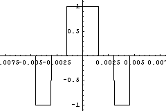
Figure 1. Step function.
|
A composite
waveform can be analyzed and described in a more simple way in order to be
processed and reproduced. Fourier Analysis is a method that gives us this
opportunity by summing infinite sine and cosine functions. It is therefore
possible, for a waveform defined on an interval (-π, π) to find the frequencies that exist in this and their widths, so that
the waveform can be described by the sum of:
The amplitudes for each frequency fn=nf, where f
is the fundamental
frequency, are given by:

|
|
As an example we can consider the step function shown in
Figure 1 where the vertical axis represents amplitude and the horizontal time. In
Figures 2, 3 and 4 are shown the cosine functions involved to synthesize the
step function of Figure 1 and in Figure 5 the sum of these three functions. In
this example the series is finite (sum of three cosine) and for this can be distinguished
differences in the form between the step function and function calculated by
the Fourier analysis.
It ispossible to use electronic devices in order a waveform can be displayed in the
form of electrical signal. Since the waveform has been analyzed in a sum of
sines and cosines, and have been calculated the frequencies and amplitudes,
electronic circuits can be designed to synthesize these frequencies and
aggregate them. The resulting electrical signal is identical to the waveform
and the differences between them are minimized as increase the terms of the
sum. The
electronic device used in this project as a generator to generate waveforms
based on a FPGA
which operates in combination with a Digital to Analog Converter (DAC). The
operating principle of the device based on digital synthesis and summation of
frequencies in FPGA.
|

Figure 5. Aggrigate of functions.
|
|

Figure 2. Cosine function f=220Hz.
|

Figure 3. Cosine function f=1100Hz.
|
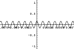
Figure 4. Cosine function f=1540Hz.
|
|
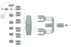
Figure 6. Basic design of Waveform Generator
|
The generated
waveform is a sum of sines, cosines and constant terms, according to the
Fourier series shown above. Sines and cosines are generated in separate
generators each, which are sequential circuits, and the constant term is given
as arithmetic value and can be customized. The design based on digital
summation of terms of the sum. The number of terms is restricted by the size of
the registers and the area of the FPGA. The size of
the registers, and therefore the terms of the sum, can be changed depending on
the needs of the waveform.
In the block
diagram of Figure 6 presented the components of the generators. The system
clock (50 MHz) clocks a counter (Counter), which compares the current value
with a constant (Constant). With this arrangement implemented a frequency divider
(System Frequency Divider). DCMs was not been used for the generation of the
frequencies used in frequency dividers, because system architecture needs
simultaneously more different frequencies from those that can generate the
DCMs. There is opportunity, depending on the hardware, to make use of DCMs to
generate the frequency of system clock for groups of generators to increase the
flexibility of the waveform generator.
|
|
When the
counter’s value becomes equal to the Constant, increases the wave address
counter (Address Counter) by one. The Address Counter gives the address to an array of size 1x64 elements of 8bit, where is stored one period of a sine wave with numerical values, so if it plotted, to form a complete period (Figure 7). The array’s size depends on the quality
of the waveform needed and affecting the frequencies that the generator is possible
to generate. In system architecture the array size affecting the size of the Address
Counters and limited by the needs of the frequencies generated for the
application and the free area of the FPGA. Addresses
0-63 of the array correspond to phase 0-2π wave. The numerical value of each element of
the table corresponds to the width of the generated voltage after conversion to
an analog signal and may be calculated by the following equation by rounding to
the nearest monad:

(Dv: The
numerical value of each element of the table, VDC: The
amplitude of the DC voltage, Vc: The
amplitude of the maximum voltage that DAC can generate, Vpp: The
voltage amplitude peak to peak of the generated wave, nm: The
number of the address of the element, Nm: The
total number of elements in the array (array size), NBit: The
number of bits of each element.)
In this example the generated wave has amplitude 1V peak to peak and a DC component with
amplitude 1.65V, if used DAC 8bit 0-3.3V. The DC component exists in the design
of the waveform generator to avoid the use of negative numbers and negative
voltages in the DAC, with reference to simpler design and space savings in the FPGA.
In Figures 8a to 8d presented snapshots from the oscilloscope’s display of four
sinusoidal waveforms generated by the waveform generator using different array
size for each.
To generate
the sum is possible to use only one array. In this case the amplitude of the
wave for each frequency involved in the aggregation will be formed by
repetition of the term. Alternatively various arrays can be made that each one
corresponds to a wave with different amplitude. These two approaches are
equivalent because they have almost the same complexity in the design, while
the space occupied in the FPGA in each case depends on the parameters of the
sum. Also is possible to use array that is stored only a quarter of period (0-π/2) since the remaining three
quarters are symmetrical in relation to this. The generation of the wave in
this case demands additional synthesis steps which increases the complexity.
These circuits included in the stage “Waveform Option” of each generator. The arrays
are the system ROM and included in stage “Waveforms”. In system architecture
selected arrays to be “Logic Vectors” so all generators can have concurrent
access to them in any address needed. This would not be possible if the tables
were stored in RAM Block.
|
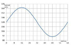
Figure 7. Period of sine
wave from array 1x64 byte.

Figure 8a. Array 1x4 Bytes.
|
|

Figure 8b. Array 1x8 Bytes.
|

Figure 8c. Array 1x16 Bytes.
|
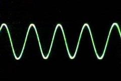
Figure 8d. Array 1x256 Bytes.
|
|
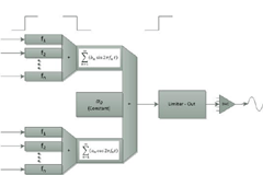
Figure 9. Adders and
registers of the waveform generator.
|
As mentioned above, each generator generates its own sine wave independently of the others.
For cosine waveforms there are not separate arrays, but the addressing of the
array is shifted by a quarter of the size of the array corresponding to π/2. The instantaneous value of each
of the wave generator is introduced into the registers f1 - fn
at the rising edge of the system clock pulse (Figure 9). These registers have
the same size with the vectors of the array (8bit in the example).
For purposes
of orderliness the series of sinus aggregated separately from the series of
cosine and each sum imported into a register at the falling edge of the system
clock pulse (Figure 9). The size of the register for each aggregation is
proportional to the number of terms of the sum, that no carry comes up from the
aggregation. If for example the sum of sines (or cosines) contains up to 16
terms of 8bit each, the register for the sum should be 12bit. In aggregation,
whereas each wave has a DC voltage and the sum must have a DC voltage too; all
proper calculations must be taken care.
The two
registers and the constant aggregated and the sum imported in the output
register at the rising edge of the system clock pulse (Figure 9). The size of
the output register depends on the constant, that no carry comes up from the
aggregation too. In the output register is useful to place a comparator - limiter,
so the amplitude of the output can be limited or updated a flag when the
amplitude exceeds certain thresholds. In this aggregation also each wave has a
DC voltage and the sum must have a DC voltage too and all proper calculations
must be taken care. Data input to registers in different phases of clock pulse
(as technical pipeline) was preferred in the design to ensure that the changes
to all logic circuits that implement the generator would be completed before
finalizing the results.
|
|
In Figures 10a
and 10b presented snapshots from the oscilloscope’s display of two different
waveforms generated from the waveform generator. The terms of the aggregation
of the waveform of Figure 10a were chosen to resemble the theoretical example of
Figure 5. For the waveform of Figure 10b the terms were chosen randomly, in
order to develop higher complexity.
Waveform generator can be used to simulate music notes. When a note
is produced by any musical instrument, the resulting sound wave contains the
fundamental frequency and also multiples of it called harmonics. Each
instrument has its own characteristic sound, so we can distinguish it from
other instruments and recognize it. This feature is called timbre or tone of
the instrument and depends on the harmonics the instrument can produce and the
intensity of each shaping in the final sound. So it is possible to determine
the frequency spectrum for each instrument and each note of it can represented with a
mathematical expression based on Fourier series. The mathematical expression then can be converted to electrical signal using the waveform
generator described above and with suitable devices (amplifier, speaker,
etc.), be converted into an acoustic signal. In Figure 11 presented the block
diagram of the modified design of the waveform generator in order to meet the
requirements of music signal synthesis as a music signal synthesizer.
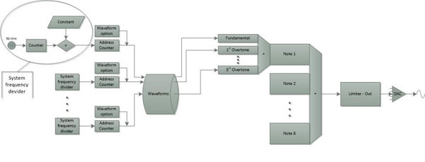
Figure 11. Basic design of the music signal synthesizer.
|

Figure 10a. Actual waveform snapshot of:
g(t)=10sin2πft +3cos2π5ft +2cos2π8ft
(f = 434Hz).

Figure 10b. Actual waveform snapshot of:
g(t)=10cos2πf1t +4cos2π2f1t +2cos2π3f1t
+4cos2π4f1t+2cos2π5f1t+4cos2π6f1t
+10sin2πf2 t +5sin2π2f2 t +3sin3πf2 t
+5sin2π4f2 t +3sin5πf2 t +5sin2π6f2 t
(f1 = 579Hz), (f2 = 434Hz).
|
|

Figure 12. The period of sinus waves as stored in arrays in the system ROM.
|
The most important modification in the system architecture is that the cosine generators were removed. Each note separately synthesized as an aggregation of sine series
consists of six harmonics, the fundamental and five overtones. The result is
input to the register of the note so that it is possible to be added to the
registers of the other notes. The registers that will be added then, and
therefore the notes will participate in the final shaping of sound, depend from
external parameter, which in this application is a key. So, there is
possibility the final sound is coming out from only one note or combination of
more notes (chords). Also adjusted a volume dampening mechanism (fade out), in
order to produce an audible effect of striking a string. In stage
Waveforms stored 9 arrays 1x64 of 8bit data. Each table can synthesize a sine
wave of fixed amplitude from 63mVpp to 1Vpp in steps of
3dB (V0 = 1mV). Figure 12 shows the graph of a period of the sinus
waves as stored in arrays in the system ROM.
The system
architecture puts some limitations, so in some cases there is deviation of the
generated fundamental frequency from the desired and its harmonics, affecting
the acoustic effect. These deviations can be eliminated within various ways,
which will be described as analyzing the limitations.
|
|
The main
limitation is the generation of a frequency with high accuracy. The frequency
of the system clock is 50MHz and a complete period of the sine wave used in the
application is composed of 64 Bytes. Therefore the maximum frequency (fm)
of a sine wave can be produced is:
fm=50·106/64=781,250Hz
Because the
frequencies of the generator generated by dividing the clock frequency with a
constant which is an integer, the frequencies that can be generated (fp)
are limited to values that gives the result of dividing the maximum frequency
with the constant:
fp=781,250/constant Hz
|
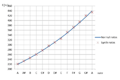
Figure 13. Deviation of the notes
synthesized by the generator.
|
|

Figure 14. Notes generated with six or four harmonics.
|
For the
synthesis of a note used six harmonics (the fundamental frequency and the first
five overtones), which are integer multiples of a frequency. Therefore, to
generate the overtones, the constants used needs to be numbers resulting from
the perfect division of the constant of fundamental frequency by the integers 2,
3, 4, 5 and 6 in order to have frequencies which are integer multiples of the
fundamental. So the minimum value that can take the constant of fundamental
frequency is the lowest common multiple of numbers 2, 3, 4, 5 and 6, which is
60 and the possible values are integer (n) multiple of 60. This limits even
more the frequencies that can be generated for the fundamental frequency (ff)
of a note:
ff=781,250/60n=13,020.833/n Hz (n
= integer)
In figure 13
presented a diagram showing the deviation of the notes of the DM scale (la major)
synthesized by the generator. This
deviation is difficult to distinguished by the human ear but becomes larger and sensate by increasing the fundamental frequency of a note (as we go higher in the musical scale).
|
|
We can reduce
or even eliminate the deviation by using some technics. Instruments do not have the same range of frequencies across the range of notes they can play. It happens, even go as high as to limit the amplitude of the higher harmonics.
This is due to vibration capability of the instrument by its manufacture, but
also constrained by devices work with the instrument. This has consequence, when musical instruments playing high notes to
change its tone and is relatively difficult to identify them. There is
therefore the possibility for high notes to not use six harmonics, but only
four. This forms the least common multiple of 60 to 12, making the number of
values that can be achieved for the fundamental frequency larger. Figure 14
shows a diagram of the notes generated with six harmonics (red marks) and with
four harmonics for the last three notes (green marks), where we can see the
deviation.
It is also
possible to use lower resolution to generate the waveforms without having such
a significant impact to their quality. Figure 8c shows that for resolution 16
Byte and more the quality of sinus waveform is satisfactory. Based on
calculations above we can conclude that for each halving of the resolution
doubles the capability of the system to produce frequencies.
|

Figure 15. Violin spectrum diagram.
|
|

Figure 16. Saxophone spectrum diagram.
|
The system
architecture allows as well for the same note different harmonics to have
different resolution. In figure 12 we can observe that as the amplitude of the
sine wave reduced, less information about its composition exists. It is
possible then, for the low amplitude sine waves to use a lower resolution,
since, anyway, there is lost information in high resolutions. And this
technique can improve the resolution of the system for generating frequencies,
increases, however, the complexity and therefore the space occupied by the
design in FPGA. Moreover is possible to use DCMs to generate the system frequency for each generator instead of the system clock (50MHz), in order to increase the flexibility of frequency generation.
According to
spectrum diagram of violin, saxophone and guitar (figure 15, 16 and 17) extracted sine series and
simulated sounds for each instrument.The sound of the violin has a constant intensity, which
depends on the pressure exerted by the musician in the chord with the bow as it
drags on. It is also possible to modify slightly the tone of the sound,depending on how the bow fits to the string.
|
|
The sound of a saxophone has a constant intensity too, which depends on the force that the
musician blows to the mouthpiece of the instrument. It is also possible to
modify greatly the tone of the sound as well, depending on how the musician blows
or depending on the material of the mouthpiece. For this reason there is
neither a specific range of frequencies nor a specific tone for the saxophone,
but both depend on the musician and is the trade mark of each one.These features can be simulated to produce the music signal synthesizer's sound similar to the sound of the violin and saxophone.
To play guitar sounds designed volume dampening mechanism (fade out), as mentioned above, which is reducing the volume as synthesized notes on generators.
To implement this operation the amplitude of the sine wave of each harmonic
decreases, based on some function of time, by selecting different array in
specific time points. The function
of time derived experimentally from the acoustic effect in combination with the image of the guitar spectrum diagram (Figure 17). Figure 18 shows a diagram
of the reduction of the amplitude of the fundamental frequency of a note in
relation to the time played that used in this application.
|
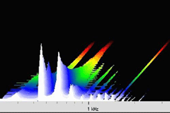
Figure 17. Guitar spectrum diagram.
|
|
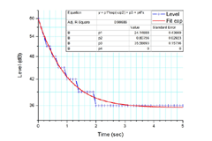
Figure 18. Fade out diagram.
|
Actually there is no specific rate, because each type of guitar has its own characteristics by
manufacture and thus there are sensate differences in sound dampening or in
tone from an instrument to another. With appropriate changes in the parameters of the waveform generator is possible to achieve appropriate sounds to coverthese differences, or even to present new features. It is also possible to incorporate in system architecture digital filters to simulate various effects used by musicians for electric guitar.
In this application modified the limiter output stage to behave like Overdrive. The Overdrive
is an effect used by guitar players very often. The operation of this effect based
on overdriving the preamp stage, in order to go to saturation. The result is to cut the tops of the sound’s waveform and becomes distorted.
Figure 19a, 19b and 19c show actual screenshots from the oscilloscope to display waveforms
corresponding to sounds from violin, saxophone and guitar, while Figure 19d shows an actual snapshot of guitar sound after the
implementation of the Digital Overdrive, as all produced from the
waveform generator.
|
|
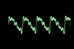
Figure 19a. Violin.
|

Figure 19b. Saxophone.
|
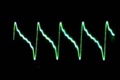
Figure 19c. Guitar.
|
|
To convertthe digital signal to analog used a simple R2R Ladder, the theoretical circuit
of which presented in Figure 20. This method causes small variations in the accuracy
of conversion and has high output impedance. These variations are not important
for the application in the developed stages. The oscilloscope used for the
impression and the device used for the amplification of the sound and playback
have also high input impedance both. For these reasons it was not necessary to
use DAC with better characteristics.
Figure 21
shows the statistics of the usage of FPGA to implement the waveform generator
and the music signal synthesizer. The implementation of the music signal synthesizer
has significantly high demands, having occupied almost the entire FPGA. The
application that exported the reports includes: eight notes with corresponding
keys, four different instruments (one of which is the guitar with the sound
damping system) with choice of two switches and four different overdrive
settings with choice of two switches too.
|

Figure 19d. Guitar with Digital Overdrive
|
|

Figure 20. R2R Ladder used for DAC.
SOURCES
-
Kendall
Milar (FAST FOURIER TRANSFORM ANALYSIS OF OBOES, OBOE REEDS AND OBOISTS: WHAT
MATTERS MOST TO TIMBRE?)
-
XILINX
-
http://www.feilding.net/
-
http://www.phy.mtu.edu/
-
http://home.cc.umanitoba.ca/
-
http://computermusicresource.com/
-
http://www.philbarone.com/blog/saxophone-news/
|
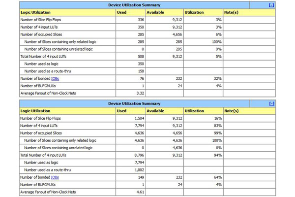
Figure 21. Statistics of the usage of FPGA, up Waveform Generator and down Music Signal Synthesizer.
|
| |
|
|


 Linkedin


